2019: Week 1 Solution
First things first, a big thanks to all who have taken part.
The response has been great and it’s good to know that this is a worthwhile initiative.
It’d be interesting to know how many of you cottoned on to the fact that Carl’s initial solution to week 1’s challenge is actually publicly visible as the
background header image on this blog!
There were a few different ways to tackle each part of this
challenge – we’ll cover a few of the possibilities for them and share two
possible workflows.
To recap, the main challenges presented were:
- Make
a date that will work in Tableau Desktop
- Work
out the total car sales per month / per car dealership
- Retain
the car sales per colour columns
Make a date that will work in Tableau Desktop
One of the easiest ways to create the date using the given
information is using of the following two functions:
- MAKEDATE(year, month, day)
- DATEADD(date_part, interval, date)
MAKEDATE() works by taking integer values for the year,
month, and day and outputting the date that corresponds to the supplied value. For
example, MAKEDATE(2018,09,01) outputs the date #2018-09-01#. So if we use our
field names instead, i.e. MAKEDATE([When Sold Year],[When Sold Month],01), we
get a nicely formatted date.
On the other hand, DATEADD() works by taking an existing
date field and adding (or subtracting!) a value from some part of it. For
example, DATEADD(‘month’, 8, #2018-01-01#) outputs the date #2018-09-01#. So if
we convert [When Sold Year] to a Date type and use DATEADD('month',[When Sold
Month]-1,[When Sold Year]), we also get a nicely formatted date. The “-1” in
the month section is important in our case as [When Sold Month] starts at “1”.
Work out the total car sales per month / per car dealership
There are two main ways to handle this:
- Use a calculated field to sum the columns.
- Pivot the data, aggregate across Date & Dealership, and join the totals back to the original date.
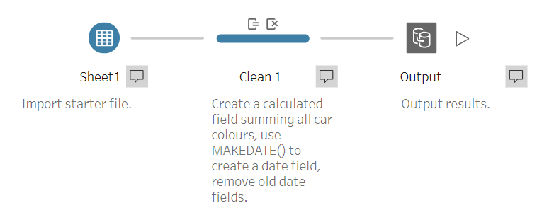
The first option is by far the quickest and retains the
individual car colour sales values with no extra work. Within a Clean step,
simply create a calculated field called “Total Cars Sold” and enter in [Red
Cars] + [Silver Cars] + [Black Cars] + [Blue Cars]. Boom, problem solved. You can
see a workflow that uses this solution below. Download here:

This works fine for a one-off report or a quick answer,
however what if we start adding more categories of cars in the future? Each
time you’d have to manually update this function. This is where the pivot &
aggregate method comes in handy, albeit at the cost of setup time.
To use the pivot & aggregate method:
2. Make sure the pivot is set to “Columns to Rows”.
3. Click where it says to use a “wildcard pivot” and type “Cars”. This is a case sensitive search, so the “C” needs to be capitalised! Hit enter, and you should see your car columns pivot into rows and a new column appear called [Cars] which contains the values for each car colour.

4. Add an Aggregation step to the right of your Pivot step.
5. Group by [Date] and [Dealership] and aggregate by the sum of
[Cars].


7. Finally, remove any duplicate fields and output the data!
You can see a full workflow using this method below. Download here:

The main danger of this method comes from the ambiguity of
the wildcard search. If another field gets added which contains “Cars” but isn’t
a type of car being sold you could be in trouble!
That's it for the first week's challenge, thanks for taking part and keep an eye out for challenge 2!


