Preppin' Data

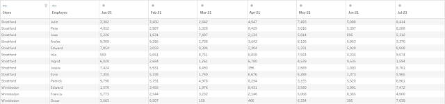
  Solution by Tom Prowse and you can download the workflow here .  This week was the final instalment of the Excel challenges month, so it seemed like the right time to involve a Vlookup and Index matches as these are such popular features. For the challenge this week we want to compare monthly targets with data stored on another sheet... let's see how we solved it! Step 1 - Average Monthly Sales The first step this week is to input the Employee Sales table and then calculate the average monthly sales for each employee.  Before using an aggregate tool to calculate the average, we need to pivot our data so that we have all of the months in a single column, therefore we can use a wildcard columns to rows pivot to bring all of the months through:  Now we have a single column for sales and months, therefore we can use the aggregation tool to calculate the average monthly sales per employee: Our table should now look like this:  Step 2 - Combine Targets & Sales We can now focus on t

 Challenge By: Jenny Martin As we come to the end of our excel challenges month, it seems only right to think about vlookups and index matches. In Excel, these are great functions for bringing together data from different worksheets without having to manually copy and paste.  Our scenario this week is looking at Employee Sales at Allchains for each month of the year so far and we want to compare this to their Monthly Targets, stored on another sheet. Inputs We have 2 inputs this week: Employee Sales Employee Targets Requirements Input data Calculate the Average Monthly Sales for each employee In the Targets sheet the Store Name needs cleaning up Filter the data so that only employees who are below 90% of their target on average remain For these employees, we also want to know the % of months that they met/exceeded their target Output the data Output 5 fields Store Employee Avg monthly Sales % of months target met Monthly Target 4 rows (5 including headers) After you finish the challeng

  Solution by Tom Prowse and you can download the workflow here . This week we continued with our Excel themed challenges by looking at how we could add some additional rows within Tableau Prep. In Excel this is easily done, but it takes some slightly different logic to achieve this in Prep so let's see how it can be done! Step 1 - Create One Data Set The first step is to create a single data source which includes all of the different files within the Input folder. Luckily these all have the same structure, therefore we can use the Wildcard Union to stack all of these on top of each other.  We want to bring through all of the files, so we use the * matching pattern to include all files After this we can remove the 'File Path' field, change the 'Table Names' to a date, then rename it to 'Reporting Date'. Finally, we are going to need the Reporting Date field twice in future steps so we can duplicate this field as well.  Our table should now look like this:  S

 Challenge by: Carl Allchin If you've spent as long as I have in the data world, you will inevitably have had moments when your sophisticated tools are actually a lot harder to solve a challenge with than Excel. The people you work with are likely to describe challenges to you in Excel terms and expect your solutions to be able to follow the same process as their logic. It's not always that easy though.  Last week when working with some client data (I've converted this to an Allchains example), my team was challenged to look at Orders captured in a weekly snapshot that was then exported into Excel.  Each week the file would show any order that was still opened that hadn't been fulfilled (ie delivered to the customer). The challenge is to classify when an order is new (the first report it has appeared in), unfulfilled (when it appears in any subsequent reports) or completed (the week after the order last appears in a report). But what if we needed to know whether the ord

  Solution by Tom Prowse and you can download the workflow here .  This week we continued with the Excel theme and focussed on the SUMIF function within Tableau Prep.  Step 1 - Flight Details After inputting the data the first task is to form the correct flight name. This is a combination of the Departure and Destination fields so we need to bring these together within a string calculation:  Flight [Departure]+ ' to '+[Destination] We can then remove the departure and destination fields and then calculate the number of days between the flight and the sales date.  Days until flight DATEDIFF('day',[Date],[Date of Flight]) Our table looks like this: Step 2 - Calculate Sales Based on Conditions Within this step we first need to classify if the sales were less or more than 7 days until the scheduled flight date. To do this we want to use the IF function to write some IF statements. First is the Less than 7 days:  Sales less than 7 days until the flight IF [Days until flight]

 Challenge by: Carl Allchin My partner is an amazing Excel user as are many of her colleagues. When in a pub, a frequent getting to know you question was "What's your favourite Excel function?". As a SQL / Tableau user, after my first meeting I knew I had to up my game. SUMIFS became my go to answer and that is one of the functions we will look to replicate in Prep this week.  SUMIF, or SUMIFS if you have multiple conditions, allows you to scan a data set and summarise the values that match any condition you create. When working with large tables with multiple entries per category, this is a great way to create some totals to help you analyse the data set. Whilst SUMIF doesn't exist within Prep, the IF function and aggregation step can be used to create the same effect.  Excel allows for lots of different types of aggregations so whilst SUMIF was my go-to answer: average, minimum, count etc are all possible too.  The challenge this week is forming the logic in Prep t

Solution by Tom Prowse and you can download the workflow here .  This week we are looking at a technique that is ubiquitous within Excel - the Pivot Table. We again re-visit the Allchains bike store and look restructuring a sales table across different items and stores. Step 1 - Remove Returns  After we have input our data set, the first step is to remove any rows that contain returns. These are documented in the 'Status' field with a 'Return to Manufacturer', so we can right-click on this in the Profile Pane and then Exclude.  Whilst we are here, we can tidy the table up a little bit. We aren't going to be using the Status or Date fields so we can remove these fields as well. Our table should now look like this:  Step 2 - Total Items Sold per Store Next we want to find the total items sold for each store. This can be achieved by using a Fixed LOD calculation, where we group by store and sum the number of items:  As a result we have got the total number of items eac

 Challenge by: Carl Allchin      When you are working with data in most organisations, you will frequently come across requests from Excel users using Excel terms. This week's challenge looks at term that is ubiquitous with Excel - a pivot table.  Pivot tables are often contain summarised data values, have totals and filter out certain parts of the data set. The challenge this week will be to take an input and create a pivot table. Pivot tables are likely to be structured differently to most of our analytical outputs. Input  The weekly sales of Bike Components from Preppin's bike store Allchains is what we are analysing. The returns are where the product has been deemed faulty before it's sold.  Requirements Input data Remove the 'Return to Manufacturer' records Create a total for each Store of all the items sold ( help ) Aggregate the data to Store sales by Item Output the data Output 6 columns: Items sold per store Wheels Tyres Saddles Brakes Store 4 rows of data

  Solution by Tom Prowse and you can download the workflow here .  Step 1 - Create TripID The first step is to create a tripID using the time of day and the date (12th July 2021). We can use a MAKEDATETIME function here. Time MAKEDATETIME( MAKEDATE(2021,7,12), MAKETIME([Hour],[Minute],0) ) Now we have the time of day that the lift made a journey, we can use a Row Number to get our tripID: TripID   {ORDERBY [Time] ASC : ROW_NUMBER()} As a result we now have our TripID for each journey made:  Step 2 - Calculate Floors Between Trips Next we need to calculate how many floors are between each trip. Before we do that, we need to categorise whether the floor is numerical or a letter (B, G), so we use an aggregate tool to return a list of the floors by just grouping by Floor:  Now we want to distinguish whether a floor is numerical or a letter. We can just do this manually by selecting the B & G, but if we wanted an automate way of categorising these we can use the following calculation: