2019: Week 22 Solution
You can view our full solution workflow below and download it here!
This week we were working on recreating another table calculation – this time to moving average. This specifically example recreates the following Tableau Desktop settings:
For each date in our data this provides us with a 1 week moving average which uses the current days sales & the past 6 days of sales and returns NULL for any date that doesn’t have at least 6 previous days.
There are 4 stages to our workflow:
In order to calculate our moving average we need to join the data to itself under the following conditions:
I’ll explain why in a little bit and first confirm how to get this [Past Date]. Here [Past Date] refers to 6 days into the past for each [Date]. In order to achieve this we can use the DATEADD() as follows:
This simply subtracts ‘6’ days from each [Date]. I’ve wrapped mine inside a DATE() function just to prevent it from generating time data that we don’t need. We also need the [Date] field to exist in two different steps so we can join it to itself later, so we also need to add a second clean step in. The [Past Date] function can exist inside the second clean step to minimise the amount of data.
For each [Date] we now need to attach 7 days worth of sales: the six days in the past and the current date. We can do this using a join with the conditions mentioned above.
Condition 1 means that each date on the RHS (right-hand-side) of the equation must be less than or equal to the date on the LHS of the equation. This prevents any future days’ sales being attached to each LHS (left-hand-side) [Date].
Condition 2 means that each date on the RHS of the equation must also be greater than or equal to the [Past Date] on the LHS. This prevents any sales from more than 6 days ago from being attached to each LHS [Date].
After this join we should now have 7 rows for each [Date] APART FROM the first 6 days in the data set which have 1-6 rows. We can delete the [Date-1] and [Past Date] fields at this point and rename [Sales-1] to [Past Sales].
Now we can simply use an aggregate step with the following conditions to generate our 1-week moving average:
 |
| The full workflow solution. |
This week we were working on recreating another table calculation – this time to moving average. This specifically example recreates the following Tableau Desktop settings:
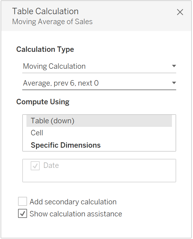 |
| Tableau Desktop moving average settings. |
For each date in our data this provides us with a 1 week moving average which uses the current days sales & the past 6 days of sales and returns NULL for any date that doesn’t have at least 6 previous days.
There are 4 stages to our workflow:
- Duplicate the data and subtract 6 days from each date.
- Join the duplicated days together so each date now has 7 rows; one for each day being used in the average.
- Aggregating to calculate the average.
- Adding NULLS where appropriate and rounding the results.
Duplicating data and subtracting 6 days from each date
 |
| The duplication and date calc section. |
In order to calculate our moving average we need to join the data to itself under the following conditions:
- [Date] >= [Date]
- [Past Date] <= [Date]
I’ll explain why in a little bit and first confirm how to get this [Past Date]. Here [Past Date] refers to 6 days into the past for each [Date]. In order to achieve this we can use the DATEADD() as follows:
|
[Past Date]
|
|
DATE(
DATEADD('day',-6,[Date])
)
|
This simply subtracts ‘6’ days from each [Date]. I’ve wrapped mine inside a DATE() function just to prevent it from generating time data that we don’t need. We also need the [Date] field to exist in two different steps so we can join it to itself later, so we also need to add a second clean step in. The [Past Date] function can exist inside the second clean step to minimise the amount of data.
Joining the data to itself
 |
| The join section. |
Condition 1 means that each date on the RHS (right-hand-side) of the equation must be less than or equal to the date on the LHS of the equation. This prevents any future days’ sales being attached to each LHS (left-hand-side) [Date].
Condition 2 means that each date on the RHS of the equation must also be greater than or equal to the [Past Date] on the LHS. This prevents any sales from more than 6 days ago from being attached to each LHS [Date].
After this join we should now have 7 rows for each [Date] APART FROM the first 6 days in the data set which have 1-6 rows. We can delete the [Date-1] and [Past Date] fields at this point and rename [Sales-1] to [Past Sales].
 |
| A snapshot of the results, showcasing 7 rows for a specific date. |
Aggregating to calculate the average sales.
Now we can simply use an aggregate step with the following conditions to generate our 1-week moving average:- GROUP BY: [Date]
- GROUP BY: [Sales]
- SUM: Number of Rows (Aggregated)
- AVG: [Past Sales]
Adding NULLS where appropriate and rounding the results.
Finally, we can use one more calculated field to both NULL the moving average if less than 7 days of [Sales] were used and round the results to two decimal places otherwise:|
[Moving Avg Sales]
|
|
IF [Number of Rows
(Aggregated)] < 7 //If less than 7
days were used…
THEN NULL //then
return NULL…
ELSE ROUND([Past Sales],2) //else round the results to 2dp.
END
|


