This week we continued our Departmental December challenges with a focus on the Sales department and a data set that doesn't have much consistency in it's format.
Step 1 - Input Data
The first step is to input the data from both sheets in the input (October & November). As they have a similar structure then we can use the wildcard union within the input tool to bring both in at the same time.
Our table should now look like this:
Step 2 - Fill In Salesperson Name
The next task is probably the most tricky throughout the whole challenge. This is to fill in the missing values within the Salesperson Name field, by 'filling' upwards because the name is at the bottom of each monthly group. We provided a hint within the requirements, so if you are stuck then make sure you take a look at that first!
In order to fill in the missing names, we first need to create a unique row ID for each of the rows. Although we already have a row ID within each of our monthly tables, we need to have a row ID across both of the tables, therefore we can create one using the following analytical calculation:
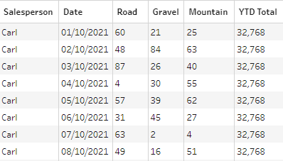
This has now created a row ID from 1 to 315, and we can remove the other Row ID & F8 fields. Our table should now look like this:
The next step is to create a self join from the step where we have just created the unique row ID. To do this we can create a new step, then within this step we want to only return rows where there is a Salesperson Name (ie. Exclude Nulls from the Salesperson field). Then remove any other fields so that we are left with the Salesperson and the Unique Row ID fields.
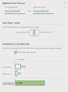
We're now ready to create the self join from the two previous steps. The join condition is based on the Unique Row ID (from the first step) <= Unique Row ID (from the second step):
This technique creates duplication within the data set, but we can then use this to fill in the missing values. You can see what is occurring by using the bar chart representations within the profile pane:
Now we have padded out the data, we need to find the first row ID for each Unique Row ID. This will give us the row where the Salesperson name is located. To do this we can use a Fixed LOD calculation:
Next we want to filter where the min row ID (Salesperson name) is equal to the Unique RowID-1 field. This will only return the rows that we require without the duplication. Note there were 315 rows in our input and after the filter we again have 315 rows.
There are a few values that contain the YTD Total label, therefore we want to remove these by removing any rows where there is a Null Date.
Our table should now look like this:
Step 3 - YTD Totals
Once we have filled in the missing Salesperson names, we can then turn our focus on the YTD totals. These are within the data table, but aren't in a separate field, therefore we need to go back to the initial step that we created (before the Unique Row ID) and create a new branch from here.
In the new step, we can then filter so that we keep only the values that contain 'YTD Total' in the Total field. After the filter we can rename F8 to YTD Total and remove all other fields so that we are left with just the Salesperson and YTD Total:
We're now ready to join this back onto our original workflow using an left-inner join on Salesperson:
The join condition wants to retain all of the rows from the original workflow (where we filled in the Salesperson names) so depending on how you set the join up this will be a left/right inner join:
As this is only YTD totals from the October table, we now need to calculate the YTD for November as well.
First we need to ensure that the YTD Total is a number, and then we can use a Fixed LOD to calculate the Monthly Total for each Salesperson:
Now we have the monthly totals for both October and November then we can use the following calculation to update the YTD totals:
YTD Total
IF [Table Names]="November"
THEN [Monthly Total]+[YTD Total]
ELSE [YTD Total]
END
We can then remove the Total, Monthly Total, and Table Names fields so that our table looks like this:
Step 4 - Prepare for Output
The final step this week is to transform the data so that we have a single column for each bike type. We can create this by pivoting the name using a Columns to Rows pivot:
You can also post your solution on the Tableau Forum where we have a Preppin' Data community page. Post your solutions and ask questions if you need any help!
Free isn't always a good thing. In data, Free text is the example to state when proving that statements correct. However, lots of benefit can be gained from understanding data that has been entered in Free Text fields. What do we mean by Free Text? Free Text is the string based data that comes from allowing people to type answers in to systems and forms. The resulting data is normally stored within one column, with one answer per cell. As Free Text means the answer could be anything, this is what you get - absolutely anything. From expletives to slang, the words you will find in the data may be a challenge to interpret but the text is the closest way to collect the voice of your customer / employee. The Free Text field is likely to contain long, rambling sentences that can simply be analysed. If you count these fields, you are likely to have one of each entry each. Therefore, simply counting the entries will not provide anything meaningful to your analysis. The value is in ...
Created by: Carl Allchin Welcome to a New Year of Preppin' Data challenges. For anyone new to the challenges then let us give you an overview how the weekly challenge works. Each Wednesday the Preppin' crew (Jenny, myself or a guest contributor) drop a data set(s) that requires some reshaping and/or cleaning to get it ready for analysis. You can use any tool or language you want to do the reshaping (we build the challenges in Tableau Prep but love seeing different tools being learnt / tried). Share your solution on LinkedIn, Twitter/X, GitHub or the Tableau Forums Fill out our tracker so you can monitor your progress and involvement The following Tuesday we will post a written solution in Tableau Prep (thanks Tom) and a video walkthrough too (thanks Jenny) As with each January for the last few years, we'll set a number of challenges aimed at beginners. This is a great way to learn a number of fundamental data preparation skills or a chance to learn a new tool — New Year...
Challenge by: Robbin Vernooij Recently, one of the Data School Coaches, Robbin, set the following challenge. It seemed perfect for a Preppin' Data, so over to Robbin: We'd like to get historical data on the highest paid athletes so we can do temporal analysis. Lucky us, it turns out Wikipedia has been tracking the Forbes list of the world's highest-paid athletes. Unlucky us, it is in an HTML table format with human readable symbols and table by table basis. Now it's time for you to clean it up into one single dataset, so that it's ready for analysis. Inputs The data for this challenge comes from this Wikipedia page . There is a table for each year that looks like this (2024 example): As well as a source table: Requirements Input the data Bring all the year tables together into a single table Merge any mismatched fields (there should not be any Null values) Create a numeric Year field Clean up the fields with the monetary amounts One way of doing this could ...